



8
月
在社区成长 8 月
LEVEL 30
100 XP
过去几年,扩散模型在图像合成方面表现出了强大的成果。现在,研究界开始致力于一项更艰巨的任务——使用它来生成视频。该任务本身是图像情况的超集,因为图像是1 帧的视频,并且更具挑战性,因为:
它对跨帧的时间一致性有额外的要求,这自然需要将更多的世界知识编码到模型中。
与文本或图像相比,收集大量高质量、高维视频数据更加困难,更不用说文本视频对了。
 必读: 请确保您已阅读之前的博客“什么是扩散模型?”在继续此处之前进行图像生成。
$$
q(\mathbf{z}_t \vert \mathbf{x})=\mathcal{N}(\mathbf{z}_t; \alpha_t \mathbf{x}, \sigma^2_t\mathbf{I})
$$
为了将$q(\mathbf{z}_t \vert \mathbf{z}_s)$ 表示为$0 \leq s t \leq T$,我们有:
$$
\开始{对齐}
\mathbf{z}_t=\alpha_t \mathbf{x} + \sigma_t\boldsymbol{\epsilon}_t \\
\mathbf{z}_s=\alpha_s \mathbf{x} + \sigma_s\boldsymbol{\epsilon}_s \\
\mathbf{z}_t=\alpha_t \Big(\frac{\mathbf{z}_s - \sigma_s\boldsymbol{\epsilon}_s}{\alpha_s}\Big) + \sigma_t\boldsymbol{\epsilon}_t \\
\mathbf{z}_t=\frac{\alpha_t}{\alpha_s}\mathbf{z}_s + \sigma_t\boldsymbol{\epsilon}_t - \frac{\alpha_t\sigma_s}{\alpha_s} \boldsymbol{\epsilon}_s \\
\text{因此}q(\mathbf{z}_t \vert \mathbf{z}_s)=\mathcal{N}\Big(\mathbf{z}_t; \frac{\alpha_t}{\alpha_s}\mathbf{z}_s, \big(1 - \frac{\alpha^2_t\sigma^2_s}{\sigma^2_t\alpha^2_s}\big)\sigma^2_t \mathbf{I}\Big)
\结束{对齐}
$$
令对数信噪比为$\lambda_t=\log[\alpha^2_t/\sigma^2_t]$,我们可以表示DDIM (Song et al. 2020) 更新为:
$$
q(\mathbf{z}_t \vert \mathbf{z}_s)=\mathcal{N}\Big(\mathbf{z}_t; \frac{\alpha_t}{\alpha_s}\mathbf{z}_s, \sigma^2_{t\vert s} \mathbf{I}\Big) \quad
\text{其中}\sigma^2_{t\vert s}=(1 - e^{\lambda_t - \lambda_s})\sigma^2_t
$$
Salimans Ho (2022) 提出了一种特殊的$\mathbf{v}$ 预测($\mathbf{v}=\alpha_t \boldsymbol{\epsilon} - \sigma_t \mathbf{x}$) 参数化。与$\boldsymbol{\epsilon}$ 参数化相比,它已被证明有助于避免视频生成中的颜色偏移。
$\mathbf{v}$ 参数化是通过角坐标中的技巧导出的。首先,我们定义$\phi_t=\arctan(\sigma_t/\alpha_t)$,因此我们有$\alpha_\phi=\cos\phi、\sigma_t=\sin\phi、\mathbf{z}_\phi=\cos\phi \mathbf{x} + \sin\phi\boldsymbol{\epsilon}$。 $\mathbf{z}_\phi$ 的速度可以写为:
$$
\mathbf{v}_\phi=\nabla_\phi \mathbf{z}_\phi=\frac{d\cos\phi}{d\phi} \mathbf{x} + \frac{d\sin\phi}{d\phi}\boldsymbol{\epsilon}=\cos\phi\boldsymbol{\epsilon} -\sin\phi\mathbf{x}
$$
那么我们可以推断,
$$
\开始{对齐}
\sin\phi\mathbf{x}
=\cos\phi\boldsymbol{\epsilon} - \mathbf{v}_\phi \\
=\frac{\cos\phi}{\sin\phi}\big(\mathbf{z}_\phi - \cos\phi\mathbf{x}\big) - \mathbf{v}_\phi \\
\sin^2\phi\mathbf{x}
=\cos\phi\mathbf{z}_\phi - \cos^2\phi\mathbf{x} - \sin\phi \mathbf{v}_\phi \\
\mathbf{x}=\cos\phi\mathbf{z}_\phi - \sin\phi\mathbf{v}_\phi \\
\text{类似}
\boldsymbol{\epsilon}=\sin\phi\mathbf{z}_\phi + \cos\phi \mathbf{v}_\phi
\结束{对齐}
$$
DDIM更新规则相应更新,
$$
\开始{对齐}
\mathbf{z}_{\phi_s}
=\cos\phi_s\hat{\mathbf{x}}_\theta(\mathbf{z}_{\phi_t}) + \sin\phi_s\hat{\epsilon}_\theta(\mathbf{z}_{\phi_t}) \quad\quad{\small \text{; }\hat{\mathbf{x}}_\theta(.), \hat{\epsilon}_\theta(.)\text{ 是基于}\mathbf{z}_{\phi_t}}\\ 预测}\mathbf{x}, \boldsymbol{\epsilon}\text{ 的两个模型
=\cos\phi_s \big( \cos\phi_t \mathbf{z}_{\phi_t} - \sin\phi_t \hat{\mathbf{v}}_\theta(\mathbf{z}_{\phi_t} ) \big) +
\sin\phi_s \big( \sin\phi_t \mathbf{z}_{\phi_t} + \cos\phi_t \hat{\mathbf{v}}_\theta(\mathbf{z}_{\phi_t} ) \big) \\
={\color{red} \big( \cos\phi_s\cos\phi_t + \sin\phi_s\sin\phi_t \big)} \mathbf{z}_{\phi_t} +
{\color{green} \big( \sin\phi_s \cos\phi_t - \cos\phi_s \sin\phi_t \big)} \hat{\mathbf{v}}_\theta(\mathbf{z}_{\phi_t} ) \\
={\color{red} cos(\phi_s - \phi_t)} \mathbf{z}_{\phi_t} +
{\color{green} \sin(\phi_s - \phi_t)} \hat{\mathbf{v}}_\theta(\mathbf{z}_{\phi_t}) \quad\quad{\small \text{;三角恒等函数。}}
\结束{对齐}
$$
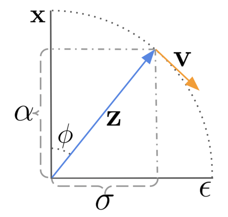 可视化扩散更新步骤如何在角坐标中工作,其中DDIM 通过沿$-\hat{\mathbf{v}}_{\phi_t}$ 方向移动$\mathbf{z}_{\phi_s}$ 来演化$\mathbf{z}_{\phi_s}$。 (图片来源: Salimans Ho, 2022)模型的$\mathbf{v}$参数化是预测$\mathbf{v}_\phi=\cos\phi\boldsymbol{\epsilon} -\sin\phi\mathbf{x}=\alpha_t\boldsymbol{\epsilon} - \sigma_t\mathbf{x}$。
在视频生成的情况下,我们需要扩散模型来运行多个上采样步骤,以延长视频长度或提高帧速率。这需要能够以第一个$\mathbf{x}^a$ 为条件对第二个视频$\mathbf{x}^b$ 进行采样,$\mathbf{x}^b \sim p_\theta(\mathbf{x}^b \vert \mathbf{x}^a)$,其中$\mathbf{x}^b$ 可能是$\mathbf{x}^a$ 的自回归扩展或者是低帧速率视频$\mathbf{x}^a$ 之间丢失的帧。
$\mathbf{x}_b$ 的采样除了其自身对应的噪声变量外,还需要以$\mathbf{x}_a$ 为条件。 Video Diffusion Models (VDM; Ho Salimans, et al. 2022) 提出了使用调整后的去噪模型的重建引导方法,使得$\mathbf{x}^b$ 的采样可以适当地以$\mathbf{x}^a$: 为条件
$$
\开始{对齐}
\mathbb{E}_q [\mathbf{x}_b \vert \mathbf{z}_t, \mathbf{x}^a]=\mathbb{E}_q [\mathbf{x}^b \vert \mathbf{z}_t] + \frac{\sigma_t^2}{\alpha_t} \nabla_{\mathbf{z}^b_t} \log q(\mathbf{x}^a \vert \mathbf{z}_t) \\
q(\mathbf{x}^a \vert \mathbf{z}_t) \approx \mathcal{N}\big[\hat{\mathbf{x}}^a_\theta (\mathbf{z}_t), \frac{\sigma_t^2}{\alpha_t^2}\mathbf{I}\big] {\small \text{;闭合形式未知。}}\\
\tilde{\mathbf{x}}^b_\theta (\mathbf{z}_t)=\hat{\mathbf{x}}^b_\theta (\mathbf{z}_t) - \frac{w_r \alpha_t}{2} \nabla_{\mathbf{z}_t^b} \| \mathbf{x}^a - \hat{\mathbf{x}}^a_\theta (\mathbf{z}_t) \|^2_2 {\small \text{;调整后的去噪模型}\mathbf{x}^b}
\结束{对齐}
$$
其中$\hat{\mathbf{x}}^a_\theta (\mathbf{z}_t), \hat{\mathbf{x}}^b_\theta (\mathbf{z}_t)$ 是去噪模型提供的$\mathbf{x}^a, \mathbf{x}^b$ 的重建。而$w_r$是一个权重因子,发现较大的$w_r 1$可以提高样本质量。请注意,还可以使用相同的重建指导方法同时对低分辨率视频进行调节,以将样本扩展为高分辨率。
VDM(Ho Salimans 等人,2022)采用标准扩散模型设置,但具有适合视频建模的更改架构。它将2D U-net 扩展为适用于3D 数据(Cicek et al. 2016),其中每个特征图代表帧x 高度x 宽度x 通道的4D 张量。此3D U 网在空间和时间上进行分解,这意味着每一层仅在空间或时间维度上运行,但不能同时在两者上运行:
处理空间:
2D U-net 中的每个旧2D 卷积层都扩展为仅空间3D 卷积;准确地说,3x3 卷积变成了1x3x3 卷积。
每个空间注意力块仍然作为空间注意力,其中第一个轴(帧)被视为批量维度。
处理时间:
在每个空间注意块之后添加时间注意块。它对第一个轴(帧)进行关注,并将空间轴视为批量维度。相对位置嵌入用于跟踪帧的顺序。时间注意力块对于模型捕获良好的时间一致性非常重要。
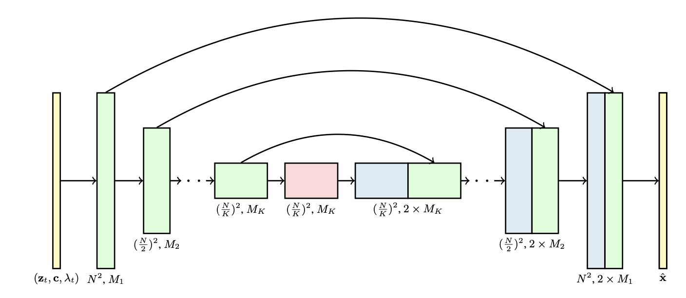 3D U-net 架构。噪声视频$\mathbf{z}_t$ 、条件信息$\boldsymbol{c}$ 和对数信噪比(log-SNR) $\lambda_t$ 是网络的输入。通道乘数$M_1, \dots, M_K$ 表示跨层的通道数。 (图片来源: Salimans Ho,2022)Imagen Video(Ho 等人,2022)基于一系列扩散模型构建,以提高视频生成质量并升级为以24 fps 输出1280x768 视频。 Imagen Video架构由以下组件组成,总共7个扩散模型。
冻结的T5 文本编码器,提供文本嵌入作为
它对跨帧的时间一致性有额外的要求,这自然需要将更多的世界知识编码到模型中。
与文本或图像相比,收集大量高质量、高维视频数据更加困难,更不用说文本视频对了。
必读: 请确保您已阅读之前的博客“什么是扩散模型?”在继续此处之前进行图像生成。从头开始视频生成建模#
首先,让我们回顾一下从头开始设计和训练扩散视频模型的方法,这意味着我们不依赖于预先训练的图像生成器。参数化采样基础知识#
这里我们使用的变量定义与上一篇文章略有不同,但数学保持不变。令$\mathbf{x} \sim q_\text{real}$ 为从真实数据分布中采样的数据点。现在我们及时添加少量高斯噪声,创建一系列$\mathbf{x}$ 的噪声变化,表示为$\{\mathbf{z}_t \mid t=1 \dots, T\}$,噪声量随着$t$ 的增加而增加,最后的$q(\mathbf{z}_T) \sim \mathcal{N}(\mathbf{0}, \mathbf{I})$。加噪前向过程是高斯过程。让$\alpha_t, \sigma_t$ 定义高斯过程的可微噪声表:$$
q(\mathbf{z}_t \vert \mathbf{x})=\mathcal{N}(\mathbf{z}_t; \alpha_t \mathbf{x}, \sigma^2_t\mathbf{I})
$$
为了将$q(\mathbf{z}_t \vert \mathbf{z}_s)$ 表示为$0 \leq s t \leq T$,我们有:
$$
\开始{对齐}
\mathbf{z}_t=\alpha_t \mathbf{x} + \sigma_t\boldsymbol{\epsilon}_t \\
\mathbf{z}_s=\alpha_s \mathbf{x} + \sigma_s\boldsymbol{\epsilon}_s \\
\mathbf{z}_t=\alpha_t \Big(\frac{\mathbf{z}_s - \sigma_s\boldsymbol{\epsilon}_s}{\alpha_s}\Big) + \sigma_t\boldsymbol{\epsilon}_t \\
\mathbf{z}_t=\frac{\alpha_t}{\alpha_s}\mathbf{z}_s + \sigma_t\boldsymbol{\epsilon}_t - \frac{\alpha_t\sigma_s}{\alpha_s} \boldsymbol{\epsilon}_s \\
\text{因此}q(\mathbf{z}_t \vert \mathbf{z}_s)=\mathcal{N}\Big(\mathbf{z}_t; \frac{\alpha_t}{\alpha_s}\mathbf{z}_s, \big(1 - \frac{\alpha^2_t\sigma^2_s}{\sigma^2_t\alpha^2_s}\big)\sigma^2_t \mathbf{I}\Big)
\结束{对齐}
$$
令对数信噪比为$\lambda_t=\log[\alpha^2_t/\sigma^2_t]$,我们可以表示DDIM (Song et al. 2020) 更新为:
$$
q(\mathbf{z}_t \vert \mathbf{z}_s)=\mathcal{N}\Big(\mathbf{z}_t; \frac{\alpha_t}{\alpha_s}\mathbf{z}_s, \sigma^2_{t\vert s} \mathbf{I}\Big) \quad
\text{其中}\sigma^2_{t\vert s}=(1 - e^{\lambda_t - \lambda_s})\sigma^2_t
$$
Salimans Ho (2022) 提出了一种特殊的$\mathbf{v}$ 预测($\mathbf{v}=\alpha_t \boldsymbol{\epsilon} - \sigma_t \mathbf{x}$) 参数化。与$\boldsymbol{\epsilon}$ 参数化相比,它已被证明有助于避免视频生成中的颜色偏移。
$\mathbf{v}$ 参数化是通过角坐标中的技巧导出的。首先,我们定义$\phi_t=\arctan(\sigma_t/\alpha_t)$,因此我们有$\alpha_\phi=\cos\phi、\sigma_t=\sin\phi、\mathbf{z}_\phi=\cos\phi \mathbf{x} + \sin\phi\boldsymbol{\epsilon}$。 $\mathbf{z}_\phi$ 的速度可以写为:
$$
\mathbf{v}_\phi=\nabla_\phi \mathbf{z}_\phi=\frac{d\cos\phi}{d\phi} \mathbf{x} + \frac{d\sin\phi}{d\phi}\boldsymbol{\epsilon}=\cos\phi\boldsymbol{\epsilon} -\sin\phi\mathbf{x}
$$
那么我们可以推断,
$$
\开始{对齐}
\sin\phi\mathbf{x}
=\cos\phi\boldsymbol{\epsilon} - \mathbf{v}_\phi \\
=\frac{\cos\phi}{\sin\phi}\big(\mathbf{z}_\phi - \cos\phi\mathbf{x}\big) - \mathbf{v}_\phi \\
\sin^2\phi\mathbf{x}
=\cos\phi\mathbf{z}_\phi - \cos^2\phi\mathbf{x} - \sin\phi \mathbf{v}_\phi \\
\mathbf{x}=\cos\phi\mathbf{z}_\phi - \sin\phi\mathbf{v}_\phi \\
\text{类似}
\boldsymbol{\epsilon}=\sin\phi\mathbf{z}_\phi + \cos\phi \mathbf{v}_\phi
\结束{对齐}
$$
DDIM更新规则相应更新,
$$
\开始{对齐}
\mathbf{z}_{\phi_s}
=\cos\phi_s\hat{\mathbf{x}}_\theta(\mathbf{z}_{\phi_t}) + \sin\phi_s\hat{\epsilon}_\theta(\mathbf{z}_{\phi_t}) \quad\quad{\small \text{; }\hat{\mathbf{x}}_\theta(.), \hat{\epsilon}_\theta(.)\text{ 是基于}\mathbf{z}_{\phi_t}}\\ 预测}\mathbf{x}, \boldsymbol{\epsilon}\text{ 的两个模型
=\cos\phi_s \big( \cos\phi_t \mathbf{z}_{\phi_t} - \sin\phi_t \hat{\mathbf{v}}_\theta(\mathbf{z}_{\phi_t} ) \big) +
\sin\phi_s \big( \sin\phi_t \mathbf{z}_{\phi_t} + \cos\phi_t \hat{\mathbf{v}}_\theta(\mathbf{z}_{\phi_t} ) \big) \\
={\color{red} \big( \cos\phi_s\cos\phi_t + \sin\phi_s\sin\phi_t \big)} \mathbf{z}_{\phi_t} +
{\color{green} \big( \sin\phi_s \cos\phi_t - \cos\phi_s \sin\phi_t \big)} \hat{\mathbf{v}}_\theta(\mathbf{z}_{\phi_t} ) \\
={\color{red} cos(\phi_s - \phi_t)} \mathbf{z}_{\phi_t} +
{\color{green} \sin(\phi_s - \phi_t)} \hat{\mathbf{v}}_\theta(\mathbf{z}_{\phi_t}) \quad\quad{\small \text{;三角恒等函数。}}
\结束{对齐}
$$
在视频生成的情况下,我们需要扩散模型来运行多个上采样步骤,以延长视频长度或提高帧速率。这需要能够以第一个$\mathbf{x}^a$ 为条件对第二个视频$\mathbf{x}^b$ 进行采样,$\mathbf{x}^b \sim p_\theta(\mathbf{x}^b \vert \mathbf{x}^a)$,其中$\mathbf{x}^b$ 可能是$\mathbf{x}^a$ 的自回归扩展或者是低帧速率视频$\mathbf{x}^a$ 之间丢失的帧。
$\mathbf{x}_b$ 的采样除了其自身对应的噪声变量外,还需要以$\mathbf{x}_a$ 为条件。 Video Diffusion Models (VDM; Ho Salimans, et al. 2022) 提出了使用调整后的去噪模型的重建引导方法,使得$\mathbf{x}^b$ 的采样可以适当地以$\mathbf{x}^a$: 为条件
$$
\开始{对齐}
\mathbb{E}_q [\mathbf{x}_b \vert \mathbf{z}_t, \mathbf{x}^a]=\mathbb{E}_q [\mathbf{x}^b \vert \mathbf{z}_t] + \frac{\sigma_t^2}{\alpha_t} \nabla_{\mathbf{z}^b_t} \log q(\mathbf{x}^a \vert \mathbf{z}_t) \\
q(\mathbf{x}^a \vert \mathbf{z}_t) \approx \mathcal{N}\big[\hat{\mathbf{x}}^a_\theta (\mathbf{z}_t), \frac{\sigma_t^2}{\alpha_t^2}\mathbf{I}\big] {\small \text{;闭合形式未知。}}\\
\tilde{\mathbf{x}}^b_\theta (\mathbf{z}_t)=\hat{\mathbf{x}}^b_\theta (\mathbf{z}_t) - \frac{w_r \alpha_t}{2} \nabla_{\mathbf{z}_t^b} \| \mathbf{x}^a - \hat{\mathbf{x}}^a_\theta (\mathbf{z}_t) \|^2_2 {\small \text{;调整后的去噪模型}\mathbf{x}^b}
\结束{对齐}
$$
其中$\hat{\mathbf{x}}^a_\theta (\mathbf{z}_t), \hat{\mathbf{x}}^b_\theta (\mathbf{z}_t)$ 是去噪模型提供的$\mathbf{x}^a, \mathbf{x}^b$ 的重建。而$w_r$是一个权重因子,发现较大的$w_r 1$可以提高样本质量。请注意,还可以使用相同的重建指导方法同时对低分辨率视频进行调节,以将样本扩展为高分辨率。
模型架构:3D U-Net DiT#
与文本到图像扩散模型类似,U-net 和Transformer 仍然是两种常见的架构选择。 Google 有一系列基于U-net 架构的扩散视频建模论文,而OpenAI 最近的Sora 模型则利用了Transformer 架构。VDM(Ho Salimans 等人,2022)采用标准扩散模型设置,但具有适合视频建模的更改架构。它将2D U-net 扩展为适用于3D 数据(Cicek et al. 2016),其中每个特征图代表帧x 高度x 宽度x 通道的4D 张量。此3D U 网在空间和时间上进行分解,这意味着每一层仅在空间或时间维度上运行,但不能同时在两者上运行:
处理空间:
2D U-net 中的每个旧2D 卷积层都扩展为仅空间3D 卷积;准确地说,3x3 卷积变成了1x3x3 卷积。
每个空间注意力块仍然作为空间注意力,其中第一个轴(帧)被视为批量维度。
处理时间:
在每个空间注意块之后添加时间注意块。它对第一个轴(帧)进行关注,并将空间轴视为批量维度。相对位置嵌入用于跟踪帧的顺序。时间注意力块对于模型捕获良好的时间一致性非常重要。
冻结的T5 文本编码器,提供文本嵌入作为


